One of the most famous techniques to simulate the cardiovascular system is through the use of 1D models. These are simplifications of the Navier-Stokes equations (which describe fluid behavior), resulting in systems of non-linear pressure and flow waves. According to studies, these models are a good approximation of the cardiovascular system, allowing for the in-depth study of diseases like hypertension, sclerosis, etc., with a good balance between precision and computational cost [1][2][3].
However, it turns out that in non-linear 1D models, the non-linearities are very mild within the physiological regime, so these systems can be simplified even further for clinical implementation. Denoting \(P\) and \(Q\) as pressure and flow, these systems can be linearized with respect to the diastolic state \((P^*, Q^*) = (P_D, 0)\) (where \(P_D\) is the diastolic pressure) without losing affinity with the real behavior of the system.
This results in the following system, which is much easier to work with [4]:
Where we define: \[
R = \frac{8 \pi \mu}{A_0^2}, \quad C = \frac{2 A_0 \sqrt{A_0}}{\beta}, \quad L = \frac{\rho}{A_0} \quad \text{with} \quad \beta = \frac{4 \sqrt{\pi} E h_0}{3}
\]
Which correspond to Peripheral Resistance \(R\), Compliance \(C\), and Inductance \(L\) (In reality, we still need to multiply each by the total length of the vessel \(l\) to truly represent physical quantities, but for practicality, we will call them that in this tutorial) [5].
Additionally, \(\rho\) represents blood density, \(\mu\) the viscosity, and \(A_0\) represents the area of the vessel during diastole. Also, \(E\) represents the Young’s modulus of the vessel and \(h_0\) is the arterial wall thickness at diastole.
The form of system Equation 1 corresponds to the Telegrapher’s Equations, which appear in the study of electrical transmission lines [6]. From this system, we can point out some characteristics:
The first equation is the relationship of Pressure and Flow in terms of Compliance (the same as the Windkessel model \(C \frac{dP}{dt} = Q_{in} - Q_{out}\)).
The second equation is the typical Pressure and Flow relationship in terms of Resistance (the one from \(\Delta P = RQ\)). Only in this one, the inertia term \(L\frac{dQ}{dt}\) is added (this gives more complexity, and more realism). In fact, this system is the temporal-spatial version of the 4-element Windkessel model.
This model can be decoupled by taking temporal derivatives in both equations, and we find that both \(P\) and \(Q\) satisfy a Damped Wave Equation. However, if \(L = 0\), both \(P\) and \(Q\) end up following a pure diffusion equation (both with a diffusion coefficient equal to \(\tau = \frac{1}{RC}\)). It can be seen that in this case, the system will be equivalent to the 2-element Windkessel model (but if we consider the terminal condition explained below, the system is a 3-element Windkessel).
To ensure the problem is well-posed, we need to impose boundary conditions. In mathematics, this system is called subcritical hyperbolic, which means we can only impose 2 boundary conditions: one at the left and another at the right of the artery. Generally, \(Q\) is imposed at the inlet and \(P\) at the outlet:
Inlet Condition: Flow Inlet We impose that the flow at the inlet of the artery corresponds to a measured/known flow that we denote by a periodic function \(Q_{in}(t)\): \[Q(x=0, t) = Q_{in}(t)\]
Terminal Condition: Windkessel in \(P\) When the pressure wave reaches the end of the artery, it encounters a terminal pressure (that of the arteries and capillaries in the rest of the body). This difference in pressure and the specific characteristics of the vessels (different lengths, different resistances) causes part of the wave to reflect and part of the wave to continue traveling. We can express this as: \[P(x = l,t) = P_{c}(t) + R_1 Q(x = l, t)\] Where \(R_1\) is the peripheral resistance that the pressure wave encounters at the terminal of the artery and \(P_c\) is the part of the pressure wave that continues traveling to the rest of the body. In this way, we are imposing that the flow \(Q\) and the pressure \(P\) reflected at the terminal have physiological sense with the arterial characteristics of the rest of the body.
However, the pressure \(P_c\) cannot be left free. To give physiological sense to this pressure, we ask it to satisfy the 3-element Windkessel equation: \[C_c \frac{d P_c}{dt} = Q(x=l, t) - P_c / R_2 \tag{2}\] Where \(R_2\) is the distal resistance of the external arteries and \(C_c\) is their respective Compliance.
Thus, the system is now closed and mathematically well-posed. However, to simulate the system, we would need to find \(P\) at the inlet and \(Q\) at the outlet. For this, we use the relations from the original system.
Initial condition imposed for P in the numerical solution:\[\frac{\partial P}{\partial x}(x=0, t) = - R Q(x=0, t) - L \frac{\partial Q}{\partial t}(x=0, t)\] Since the value of \(Q\) is being imposed directly at the inlet, we can use this equation to find \(P\) at the inlet (\(x=0\)).
Final condition imposed for Q in the numerical solution:\[\frac{\partial Q}{\partial x}(x=l, t) = - C \frac{\partial P(x=l)}{\partial t}\] Again, the terminal condition offers a relationship for \(P\) and \(Q\). With this new condition, we can perfectly find the values of \(P\) and \(Q\) at the border of the artery (\(x=l\)).
Now we can finally simulate the system numerically.
NOTE: For both the system Equation 1 and Equation 2, it is necessary to impose some initial condition. However, since we are really interested in the periodic state of the system (that is, analyzing how the pressure and flow variables behave in the long term), we can initialize in the diastolic state \((P, Q) = (P_D, 0)\) and simulate the system long enough to reach the periodic state. For Equation 2, we can initialize at any point (e.g., \(P_c=0\)) and still reach the same periodic state. However, later we will use a technique to reach this state more efficiently.
How do we simulate this system?
To simulate this type of models, different techniques exist in the literature:
Applying the Finite Element Method (Discontinuous Galerkin) [7].
Converting the system into a chain of Windkessels and solving each ODE (0D model chain) [4].
However, remembering that this system is a form of the telegrapher’s equations and taking advantage of the nature of waves, we are going to apply a method based on Fourier. Let’s consider the linearized 1D model again: \[
\begin{cases}
C\dfrac{\partial P}{\partial t} + \dfrac{\partial Q}{\partial x} &= 0 \\
L\dfrac{\partial Q}{\partial t} + \dfrac{\partial P}{\partial x} &= - RQ
\end{cases}
\] We take the Fourier transform with respect to time for both equations (by doing this, we are assuming that \(P\) and \(Q\) are already in the stationary period, due to the periodicity of the Fourier transform), so that we have: \[
\begin{cases}
\dfrac{\partial \hat{Q}}{\partial x} &= -i C \omega \hat{P} = -Y \hat{P} \\
\dfrac{\partial \hat{P}}{\partial x} &= - R\hat{Q} - iL \omega \hat{Q} = - Z \hat{Q}
\end{cases}
\tag{3}\] Where \(\hat{Q} = \hat{Q}(\omega, x)\) and \(\hat{P} = \hat{P}(\omega, x)\) are now functions of space and frequency.
Also, \(Z = R + i \omega L\) is known in circuits as the series impedance and \(Y = i \omega C\) is the parallel admittance.
With these variables, we can calculate the Characteristic Impedance of the artery, given by \(Z_c = \sqrt{Z / Y}\), and its Propagation Coefficient\(\gamma = \sqrt{Z Y}\).
In turn, this form allows us to considerably simplify the boundary conditions.
Inlet Condition: Flow Inlet It becomes its frequency-domain analogue: \[\hat{Q}(x=0, \omega) = \hat{Q}_{in}(\omega) \]
Terminal Condition: Windkessel in \(P\) It simply becomes: \[\hat{P}(x = l, \omega) = Z_{WK3} \hat{Q}(x = l, \omega)\] Where \(Z_{WK3}\) is the characteristic impedance of the arteries in the rest of the body, given by the formula: \[
Z_{WK3} = R_1 + \frac{R_2}{1 + i \omega R_2 C_c}
\]
If it turns out that \(Z_{WK3} = Z_c\), then the wave propagates perfectly without reflections. It is the change in impedances—that is, the fact that \(Z_{WK3} \neq Z_c\)—what causes the pressure and flow waves to reflect and deform as they travel through the arterial tree.
Returning to Equation 3, if we apply derivative with respect to \(x\) in both equations, then we can write: \[
\begin{cases}
\dfrac{\partial^2 \hat{P}}{\partial x^2} &= Z Y \hat{P} \\
\dfrac{\partial^2 \hat{Q}}{\partial x^2} &= Z Y \hat{Q}
\end{cases}
\] Which have the analytical solution: \[
P(\omega, x) = A e^{-\gamma x} + B e^{\gamma x}
\]\[
Q(\omega, x) = C e^{-\gamma x} + D e^{\gamma x}
\] For certain constants \(A, B, C\), and \(D\) (Remember that \(\gamma\) depends on the frequency \(\omega\)).
This means that \(P\) and \(Q\) are composed of a wave traveling forward (the part with \(e^{-\gamma x}\)) and another traveling backward (the one with \(e^{\gamma x}\)).
Finally, by evaluating at \(x=0, x=l\) and after some calculations, we can find that: \[
\begin{bmatrix}
\hat{P}(\omega, l) \\ \hat{Q}(\omega, l)
\end{bmatrix} =
\begin{bmatrix}
\cosh(\gamma l) & -Z_c \sinh(\gamma l) \\
-\frac{1}{Z_c}\sinh(\gamma l) & \cosh(\gamma l)
\end{bmatrix}
\begin{bmatrix}
\hat{P}(\omega, 0) \\ \hat{Q}(\omega, 0)
\end{bmatrix}
\]
This defines a Transmission Matrix, which allows us to travel from the information at \(x=0\) to the information at \(x=l\). It’s good to note that:
This transmission matrix has a determinant of 1, which reflects the principle of conservation.
To go through several segments, A -> B -> C, we can simply multiply the matrices; it is enough to consecutively apply the transmission matrix of each artery with respect to the initial state, i.e.: \[
\begin{bmatrix}
\hat{P_C}(\omega, l) \\ \hat{Q_C}(\omega, l)
\end{bmatrix} = \textbf{M}_C \textbf{M}_B \textbf{M}_A \begin{bmatrix}
\hat{P_A}(\omega, 0) \\ \hat{Q_A}(\omega, 0)
\end{bmatrix}
\]
If we want the information at an intermediate point, say an \(x\) between \(0\) and \(l\), we replace \(l\) with \(x\) in the transmission matrix formula and apply it to the data at \(x=0\).
So, this would be our strategy to simulate an artery:
We consider \(P(x=0,t)\) and \(Q(x=0,t)\) and calculate their FFT.
We calculate the transmission matrix.
We apply the transmission matrix to find \(\hat{P}(x=l,t)\) and \(\hat{Q}(x=l,t)\).
We apply IFFT, and this gives us the Pressure and Flow information at \(x=l\).
However, let’s remember that, according to the inlet conditions, we only know \(Q(x=0,t)\).
The Impedance Propagation Algorithm
To find \(P(x=0,t)\), we use the impedance relationship between Pressure and Flow at the inlet of the system: \[
\hat{P}(x=0,t) = Z_{in} \hat{Q}(x=0,t)
\] Where \(Z_{in}\) represents the characteristic impedance at the inlet of the artery, given by: \[
Z_{in} = Z_c \frac{Z_{WK3} + Z_c \tanh(\gamma l)}{Z_c + Z_{WK3} \tanh(\gamma l)}
\] So we can calculate the impedance at the beginning of the segment using the terminal condition (to calculate \(Z_{WK3}\)) and the segment’s properties (to calculate \(Z_c\) and \(\gamma\)).
In general, this formula allows calculating the impedance at the beginning of an artery (\(Z_{in}\)) when knowing the impedance at the end of it (which we call \(Z_{WK3}\)).
In this way, we have an impedance propagation algorithm that allows us to simulate the system for an entire arterial tree:
We calculate/measure the initial \(Q(x=0, t)\) and its FFT.
We calculate the impedances of the terminal nodes of the tree.
We calculate the impedances of the internal arteries of the tree, using the formula we found that relates its inlet impedance with its outlet impedance (being careful at bifurcations).
Once we have \(Z_{in}\), at the same node as \(Q(x=0, t)\), we calculate \(\hat{P}(x=0, \omega) = Z_{in} \hat{Q}(x=0, \omega)\).
Now we can use the transmission matrices of each segment to simulate pressures and flows in the rest of the tree.
What happens at bifurcations?
When we have a bifurcation, the impedances combine according to the following formula: \[
\frac{1}{Z_{parent}} = \sum \frac{1}{Z_{daughters}} \quad \text{over all daughters}
\] Here, \(Z_{parent}\) represents the impedance at the end of the parent segment, and each \(Z_{daughter}\) represents the impedance at the inlet of each daughter segment.
This formula must be taken into account both when propagating impedances backward through the tree:
First, the inlet impedances of each daughter are calculated.
Then, this formula is used to find the impedance at the end of the parent segment.
Having the impedance at the end of the parent segment, we calculate the impedance at its inlet, and so on, propagating backward until reaching the \(Q(x=0, \omega)\) node.
Additionally, when propagating \(P\) and \(Q\) forward using the transmission matrices, we must be careful upon reaching a bifurcation. At that point, we impose the so-called continuity condition:
Upon reaching a bifurcation, we impose that the pressure at the end of the parent must be equal to the pressure at the inlet of the daughters, i.e.: \[
P_{parent}(\omega, x=l) = P_{daughter1}(\omega, x=0) = \cdots = P_{daughterN}(\omega, x=0)
\] This is equivalent to: \[
\hat{P}_{parent}(\omega, x=l) = \hat{P}_{daughter1}(\omega, x=0) = \cdots = \hat{P}_{daughterN}(\omega, x=0)
\] Which is what we impose in the simulation.
In a bifurcation, we must ensure that the flow at the end of the parent is equal to the total of the flows distributed into each daughter, i.e.: \[
Q_{parent}(t, x=l) = \sum Q_{daughter}(t, x=0) \quad \text{over all daughters}
\] To achieve this, we calculate the inlet flow to each daughter from the impedance relationship, using the corresponding impedances of each daughter. That is, for each daughter, we impose: \[
\hat{Q}_{daughter}(\omega, x=0) = \frac{\hat{P}_{daughter}(\omega, x=0)}{Z_{daughter}}
\] Where \(\hat{P}_{daughter}(\omega, x=0)\) is the pressure we just calculated (which is equal to the pressure at the end of the parent segment), and \(Z_{daughter}\) are the impedances at the inlet of the corresponding daughter.
And with these relationships, we can finish simulating the arterial tree and incorporate bifurcations without any problem.
Simulation Example
Below we show step by step a simulation example using the described method.
In this case, we will replicate the Upper Thoracic Aorta (UTA) example described in [2], [7][3]. In these works, non-linear 1D models (solved using DG FEM) are used to obtain, given an inlet flow curve, the evolution of pressure at the end of the segment in one cardiac cycle. So, we start by defining the model parameters. Additionally, we calculate the resistance, compliance, and characteristic inductance of the artery.
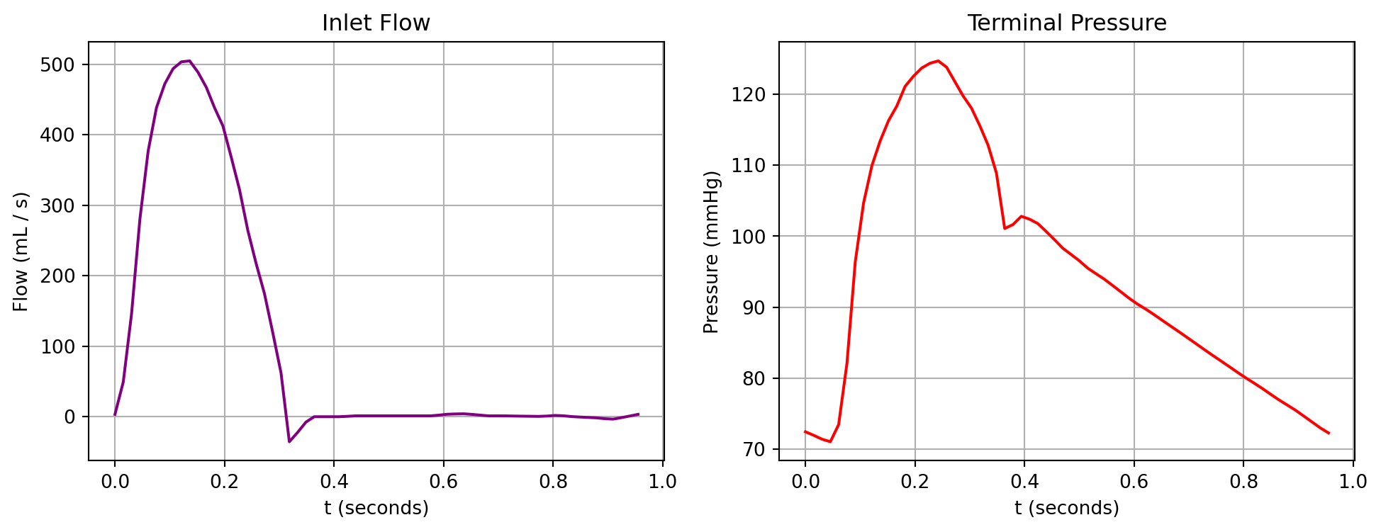
Now, we import the inlet flow data \(Q_{in}\) and the final pressure \(P_{final}\) at the end of the segment obtained through the non-linear 1D model.
Code
import pandas as pd# Load input dataQ_in_data = pd.read_csv('Q_in.csv').values.Tt_Qin = np.array([float(i.replace(',', '.')) for i in Q_in_data[0]])val_Qin = np.array([float(i.replace(',', '.')) for i in Q_in_data[1]])P_final_data = pd.read_csv('P_final.csv').values.Tt_Pf = np.array([float(i.replace(',', '.')) for i in P_final_data[0]])val_Pf = np.array([float(i.replace(',', '.')) for i in P_final_data[1]])T = t_Qin[-1]Nt =64t = np.linspace(0, T, Nt)dt = t[1] - t[0]def Q_in_func(t):return np.interp(t % t_Qin[-1], t_Qin, val_Qin) # Returns mL/sdef P_final_func(t):return np.interp(t % t_Pf[-1], t_Pf, val_Pf) *1e3/133.322# Returns mmHgplt.figure(figsize=(12, 4))plt.subplot(1, 2, 1)plt.plot(t, Q_in_func(t), color='purple')plt.xlabel("t (seconds)")plt.ylabel("Flow (mL / s)")plt.title("Inlet Flow")plt.grid()plt.subplot(1, 2, 2)plt.plot(t, P_final_func(t), color='red')plt.xlabel("t (seconds)")plt.ylabel("Pressure (mmHg)")plt.title("Terminal Pressure")plt.grid()
We define the frequency domain and calculate the characteristic impedances \(Z_c\) and the propagation coefficient \(\gamma\).We also calculate the outlet impedance \(Z_{WK3}\) (given by the Windkessel parameters at the outlet), and with it, the inlet impedance \(Z_{in}\).
Code
fs =1/ dt # [Hz]w =2* np.pi * np.fft.rfftfreq(len(t), 1/fs) # [Radians / s]w[0] =1e-12# Avoid division by zeroZ_freq = R +1j* w * L # [Pa * s / m^4]Y_freq =1j* w * C # [m^2 / (Pa * s)]gamma = np.sqrt(Z_freq * Y_freq) # [1 / m]Zc = np.sqrt(Z_freq / Y_freq) # [Pa * s / m^3]Zc[0] = Zc[1] # Avoid division by zeroZ_WK3 = R1 + R2 / (1+1j* w * R2 * Cc) # [Pa * s / m^3]Zin = Zc * (Z_WK3 + Zc * np.tanh(gamma * l)) / (Zc + Z_WK3 * np.tanh(gamma * l)) # [Pa * s / m^3]
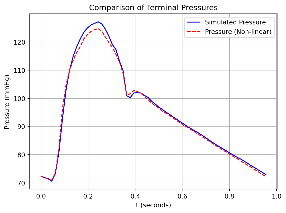
Now we calculate the FFT of the inlet flow \(Q_{in}\). With it, we calculate the FFT of the inlet pressure, and using the transmission matrix, we calculate the pressure and flow at the end of the artery.Finally, we return to the time domain by applying the IFFT and plot the results.
We notice that both curves are practically identical, with the greatest difference appearing near the systolic peak. The errors also show good affinity, with Diastolic Pressure (PD) and Mean Arterial Pressure (PAM) errors being practically negligible.
In this way, we can simulate the behavior of flow and pressure waves, maintaining a balance between fidelity and low computational cost compared to other methods.
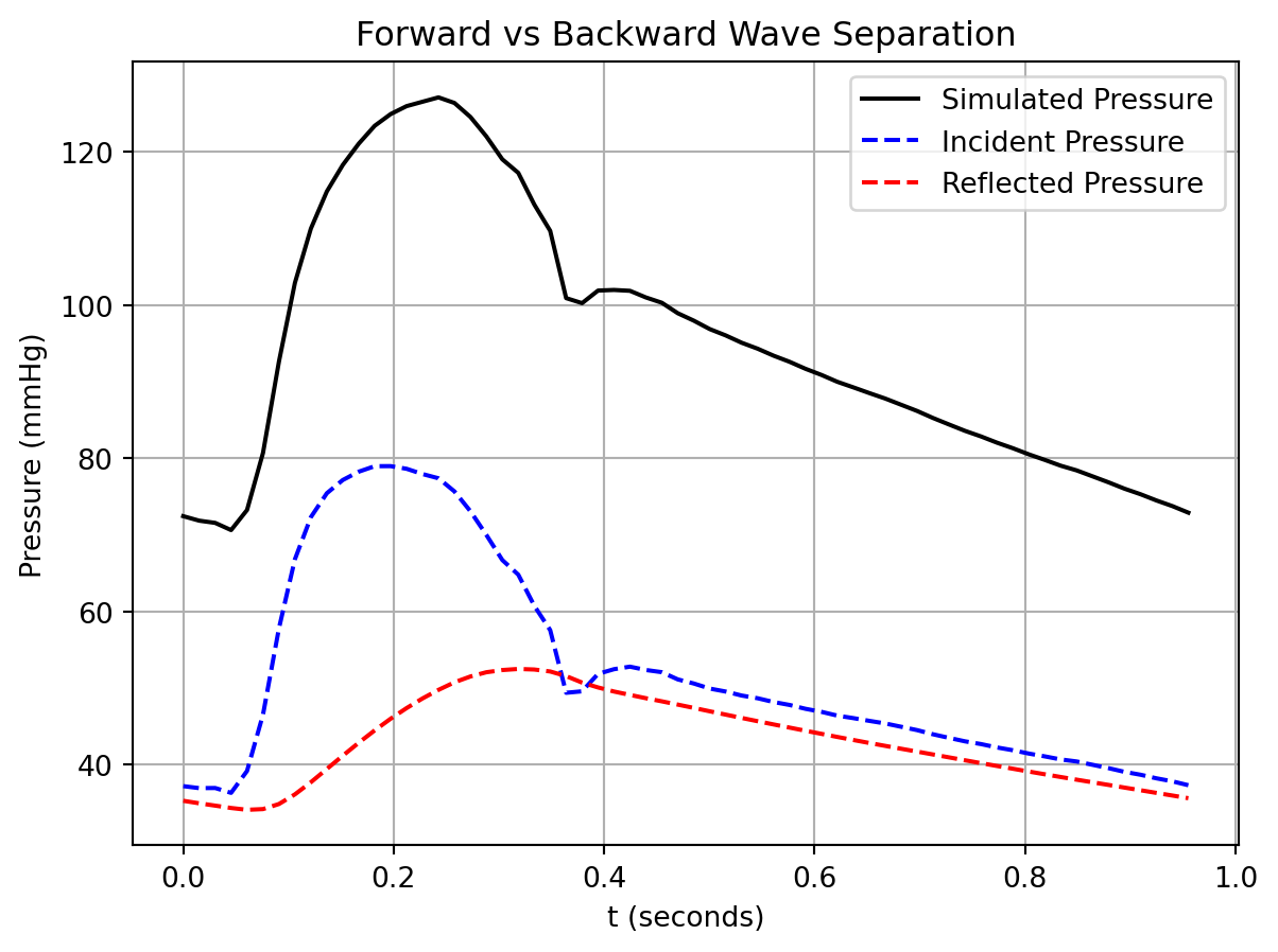
Additionally, we can plot the incident and reflected propagation waves, which helps in medical analysis.
P. Reymond, F. Merenda, F. Perren, D. Rufenacht, and N. Stergiopulos, “Validation of a one-dimensional model of the systemic arterial tree,”American Journal of Physiology-Heart and Circulatory Physiology, vol. 297, no. 1, pp. H208–H222, 2009.
[2]
E. Boileau et al., “A benchmark study of numerical schemes for one-dimensional arterial blood flow modelling,”International journal for numerical methods in biomedical engineering, vol. 31, no. 10, p. e02732, 2015.
[3]
I. Benemerito, A. Melis, A. Wehenkel, and A. Marzo, “openBF: An open-source finite volume 1D blood flow solver,”Physiological Measurement, vol. 45, no. 12, p. 125002, 2024.
[4]
V. Milišić and A. Quarteroni, “Analysis of lumped parameter models for blood flow simulations and their relation with 1D models,”ESAIM: Mathematical modelling and numerical analysis, vol. 38, no. 4, pp. 613–632, 2004.
[5]
N. Westerhof, N. Stergiopulos, and M. I. Noble, Snapshots of hemodynamics: An aid for clinical research and graduate education. Springer, 2005.
N. Xiao, J. Alastruey, and C. Alberto Figueroa, “A systematic comparison between 1-d and 3-d hemodynamics in compliant arterial models,”International journal for numerical methods in biomedical engineering, vol. 30, no. 2, pp. 204–231, 2014.